Hybrid Quantum Support Vector Machine Classifier Example

The following example details a possible implementation of a hybrid support vector classifier applied on the iris dataset.

An SVM convex optimization problem can be reformulated into a system of linear equations in the form \(Ax= b\), the solution of which is a trained SVM model: \begin{align*} \begin{bmatrix} 0 & 1^T_M \\ 1_M & K+\gamma^{-1}I_M \end{bmatrix} \begin{bmatrix} \beta \\ \alpha \end{bmatrix} = \begin{bmatrix} 0 \\ Y \end{bmatrix} \end{align*} with \(M\) number of training samples, \(K=K(x_i,x_j)\) kernel matrix, \(X\) training set, \(Y\) classification labels, \(\gamma\) regularization hyperparameter, \(1_M = [1,...1]^T\), \(I_M\) identity matrix, \(\alpha\) and \(\beta\) respectively weights and bias used in prediction. Model prediction on new data can be obtained as \begin{align*} f(\cdot) = K( \cdot,X) \cdot \alpha + \beta \end{align*}

Building \(A\) requires computing the kernel matrix \(K\) of distances from each sample to each sample, which is done in a quantum fashion, and solving the system requires a matrix inversion.

# TODO: uncomment the next line after release qlearnkit 0.2.0
#!pip install qlearnkit
!pip install matplotlib

Requirement already satisfied: matplotlib in /home/akatief/PycharmProjects/qlearnkit/.venv/lib/python3.9/site-packages (3.5.1)
Requirement already satisfied: cycler>=0.10 in /home/akatief/PycharmProjects/qlearnkit/.venv/lib/python3.9/site-packages (from matplotlib) (0.11.0)
Requirement already satisfied: python-dateutil>=2.7 in /home/akatief/PycharmProjects/qlearnkit/.venv/lib/python3.9/site-packages (from matplotlib) (2.8.2)
Requirement already satisfied: packaging>=20.0 in /home/akatief/PycharmProjects/qlearnkit/.venv/lib/python3.9/site-packages (from matplotlib) (21.3)
Requirement already satisfied: pillow>=6.2.0 in /home/akatief/PycharmProjects/qlearnkit/.venv/lib/python3.9/site-packages (from matplotlib) (9.1.0)
Requirement already satisfied: numpy>=1.17 in /home/akatief/PycharmProjects/qlearnkit/.venv/lib/python3.9/site-packages (from matplotlib) (1.21.5)
Requirement already satisfied: kiwisolver>=1.0.1 in /home/akatief/PycharmProjects/qlearnkit/.venv/lib/python3.9/site-packages (from matplotlib) (1.4.2)
Requirement already satisfied: fonttools>=4.22.0 in /home/akatief/PycharmProjects/qlearnkit/.venv/lib/python3.9/site-packages (from matplotlib) (4.32.0)
Requirement already satisfied: pyparsing>=2.2.1 in /home/akatief/PycharmProjects/qlearnkit/.venv/lib/python3.9/site-packages (from matplotlib) (3.0.8)
Requirement already satisfied: six>=1.5 in /home/akatief/PycharmProjects/qlearnkit/.venv/lib/python3.9/site-packages (from python-dateutil>=2.7->matplotlib) (1.16.0)
WARNING: You are using pip version 21.3.1; however, version 22.0.4 is available.
You should consider upgrading via the '/home/akatief/PycharmProjects/qlearnkit/.venv/bin/python -m pip install --upgrade pip' command.

import numpy as np
from qlearnkit.algorithms.qsvm import QSVClassifier
from sklearn.preprocessing import MinMaxScaler
from sklearn.datasets import load_iris
from sklearn.svm import SVC
from matplotlib import pyplot as plt
from qiskit import BasicAer
from qiskit.circuit.library import PauliFeatureMap
from qiskit.utils import QuantumInstance

Let’s first prepare our data.

# import some data to play with
iris = load_iris()
mms = MinMaxScaler()
X = iris.data[:, :2]  # we only take the first two features. We could
                      # avoid this ugly slicing by using a two-dim dataset
X = mms.fit_transform(X)
y = iris.target

Now Let’s prepare the feature map we are going to use, along with the backend we will run the simulation on.

seed = 42
encoding_map = PauliFeatureMap(2)
quantum_instance = QuantumInstance(BasicAer.get_backend('statevector_simulator'),
                                   shots=1024,
                                   optimization_level=1,
                                   seed_simulator=seed,
                                   seed_transpiler=seed)

Let’s create our quantum SVC from qlearnkit along with a classical SVC for comparison.

svc = SVC(kernel='linear')
qsvc = QSVClassifier(encoding_map=encoding_map, quantum_instance=quantum_instance)

Now we can train our hybrid-quantum model

svc.fit(X,y)
qsvc.fit(X,y)

And finally we plot the decision boundaries of the two algorithms and see how they perform

h = 0.1 # step size in the mesh
# create a mesh to plot in
x_min, x_max = X[:, 0].min() - 0.2, X[:, 0].max() + 0.2
y_min, y_max = X[:, 1].min() - 0.2, X[:, 1].max() + 0.2
xx, yy = np.meshgrid(np.arange(x_min, x_max, h),
                     np.arange(y_min, y_max, h))

# title for the plots
titles = ['SVC with linear kernel',
          'QSVC with Pauli feature map']

for i, clf in enumerate((svc, qsvc)):
    # Plot the decision boundary. For that, we will assign a color to each
    # point in the mesh [x_min, x_max]x[y_min, y_max].
    plt.subplot(2, 1, i + 1)
    plt.subplots_adjust(wspace=0.4, hspace=0.4)
    Z = clf.predict(np.c_[xx.ravel(), yy.ravel()])

    # Put the result into a color plot
    Z = Z.reshape(xx.shape)
    plt.contourf(xx, yy, Z, cmap="RdBu", alpha=0.8)

    # Plot also the training points
    plt.scatter(X[:, 0], X[:, 1], c=y, cmap="RdBu",edgecolor="grey" )
    plt.xlabel('Sepal length')
    plt.ylabel('Sepal width')
    plt.xlim(xx.min(), xx.max())
    plt.ylim(yy.min(), yy.max())
    plt.xticks(())
    plt.yticks(())
    plt.title(titles[i])

plt.show()

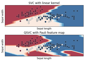
Notice how the quantum boundary is nonlinear. This is a consequence of the Pauli feature map we used. Different settings and different feature maps give different results. The choice of simulator also plays a role in how the final boundary looks like. In this example QASM - a noisy backend - was used. In case you want to try with a different backend simulator you could also use QASM (a complete list is available on the Qiskit documentation).